Geologic Layer Development

Introduction

Construction of the three-dimensional interpretation of geologic layers, and by extension hydrostratigraphic units (aquifers/aquitards), has been one of the most challenging tasks of the Oak Ridges Moraine Groundwater Program (ORMGP). This is an ongoing process whereby the geologic layers are updated as new data and conceptual understanding become available. The picking of geologic surfaces at borehole locations is a fundamental step in this process; however, to fully represent the complexity of the geologic architecture, geologic picks are supplemented with information obtained from other indicators including surficial geology mapping, geophysics (borehole methods and land-based methods such as seismic surveys), expert intuition and geologic conceptual understanding of the sedimentological processes, and hydrogeology (e.g., well screen placement, groundwater levels). This information is integrated into the geologic-model construction process using other methods such as the use of polylines (lines of geologic contact) to constrain the interpolation processes.

Database integration, data visualization, geologic layer picking and geostatistical analyses are required to review and interpret the large amounts of borehole data. The result is a three-dimensional geologic model, and by extension hydrostratigraphic model, that honours the borehole and well data and encapsulates the conceptual understanding of the processes that formed the Oak Ridges Moraine.

The geological layer construction methodology described below has been modified from the original description contained within an appendix of Earthfx Inc. (2006).

Background

Southern Ontario is underlain by Quaternary surficial sediments that can exceed 200 m in thickness. Beneath this sediment package lies Paleozoic bedrock that has a surface characterized by a series of exposed escarpments and a deep bedrock trough (Laurentian trough), including tributary bedrock valleys. In addition, there are secondary bedrock valleys that are smaller in scale. The bedrock surface was shaped by a combination of fluvial, glacial and glaciofluvial processes. The Quaternary sediments in the ORMGP study area (south-central Ontario) is a complex assemblage of alternating glacial (till, glacio-lacustrine/fluvial) and interglacial deposits, and includes regional unconformities.

Figure 1 depicts the stratigraphic framework for south-central Ontario (from Sharpe et al., 2011) depicting the approximate age, lithostratigraphy, and chronostratigraphy for the various geologic units present, including major unconformities. There are five major geologic units present within the study including (from youngest to oldest):

Surficial till units including local glaciolacustrine veneer (e.g., Halton Till);
Oak Ridges Moraine (ORM);
Newmarket Till;
Lower Sediments (including Thorncliffe Fm., Sunnybrook Drift, Scarborough Fm., and locally the Don Formation and York Till); and
Bedrock.

The ORM consists of channel and ridge sediments as part of the landform architecture that occur above the Newmarket Till, which is interpreted to occur throughout the study area. Lower Sediment comprises a series of formations and units below the Newmarket Till resting on bedrock, which are exposed in outcrops close to the Lake Ontario shore (e.g., Karrow, 1967) and extend northward for various distances. The northern extent of units is often difficult to trace due to a decrease in density of deep borehole data for the thick Quaternary sediment package beneath the Oak Ridges Moraine and above the Laurentian bedrock trough. Lower Sediments are thickest within the Laurentian trough and thin towards upland areas associated with the Canadian Shield to the north and the Niagara Escarpment to the west. Unconformities are present within the Quaternary sediment package. A major unconformity occurs beneath the Oak Ridges Moraine (ORM) due to channelization processes and subsequent infill (ORM-channels), with older local unconformities occurring within the upper part of the Lower Sediment package (Upper Thorncliffe Formation; Thorncliffe-channels). Both ages of channels are infilled with fining-upward sequences consisting of (oldest to youngest) gravel, sand, and capped by silt/clay rhythmites. Channels are very important to the hydrogeology of the study area in that they contain the highest permeability aquifer units.

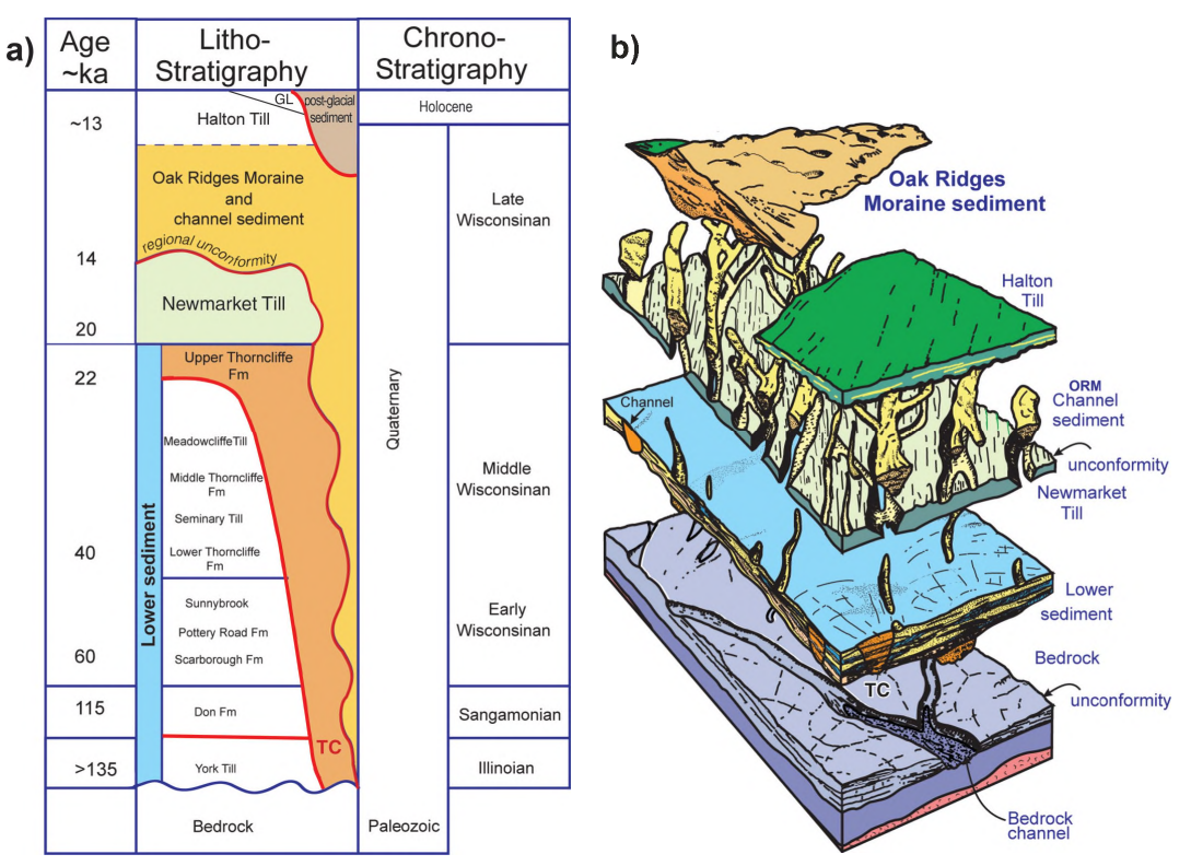*Figure 1* Figure 1: Stratigraphic Framework (modified from Sharpe et al., 2011 and included in Sharpe et al., 2018 and Gerber et al., 2018). Unconformities shown as red lines.

Figure 2 illustrates the current translation of the geologic layers to hydrostratigraphic units within the ORMGP conceptual model. This north-south cross section extends from Lake Simcoe in the north across the Oak Ridges Moraine (ORM) to Lake Ontario in the south. The main aquifer units are the ORM sediments, ORM-channel (C2), Thorncliffe Formation channels (C1), and sands of the Thorncliffe Formation and the Scarborough Formation. The main aquitard units are the glaciolacustrine/surficial diamict deposits (e.g., Halton Till), the Newmarket Till, and Lower Sediment silt, clay and diamict (e.g., Sunnybrook Drift). A groundwater divide occurs beneath the Oak Ridges Moraine in all aquifer units.

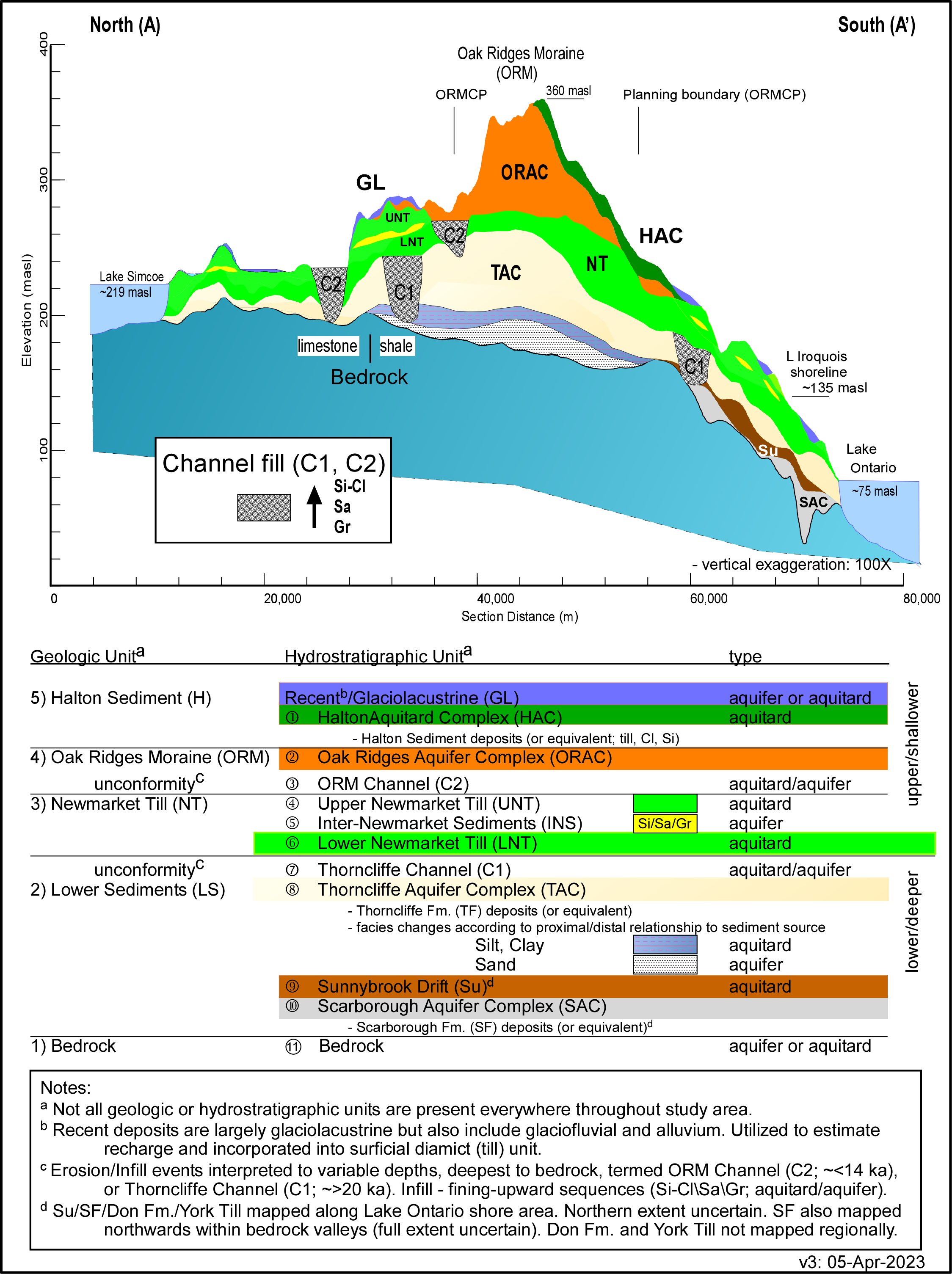*Figure 2* Figure 2: Translation of geologic layer interpretation to hydrostratigraphic layers within the ORMGP conceptual model. Hydrostratigraphic layers are units of similar hydraulic properties and hydrogeologic function, which may or may not conform to geologic layer contacts. The geologic layers, and subsequent hydrostratigraphic interpretation are subject to continual testing and refinement as more information is obtained. Comment and constructive critique are always welcome. To discuss any aspect of this interpretation please contact either Rick Gerber (rgerber@owrc.ca) or Steve Holysh (sholysh@owrc.ca).

The ORMGP three-dimensional geologic model has built upon the original interpretations of the Oak Ridges Moraine sediments undertaken during the 1990s by the Geological Survey of Canada (GSC), and researchers at southern Ontario universities. Refinement of the ORMGP geologic model occurs through ongoing discussions with geologists of the GSC, the Ontario Geological Survey (OGS), university researchers, and consultants largely through regional-scale numerical groundwater modelling projects associated with water supply and source water protection initiatives.

Data Correction and Data Biases

There is a wide range of quality and reliability of the geologic information housed within the ORMGP database from higher quality cored borehole information prepared by geologists (universities, GSC, OGS, consultants) to relatively lower quality information recorded by non-geologists collected during the well drilling process. Ontario Ministry of Environment, Conservation and Parks (MECP) well driller’s logs form the majority of the borehole information in the ORMGP database. Although the accuracy and reliability of individual wells in this data set can be questionable, the borehole logs can provide useful information about the subsurface. Borehole data is visually screened and corrected for obvious or known errors, thereby minimizing the potential biases in the driller’s logs. Water well geologic and well-construction information are largely utilized to infill areas existing between higher-quality geologic information locations.

Some of the location and elevation errors in the MECP’s database were addressed through field validation (using GPS) of over 5,000 of the wells which had not previously been located (Beatty and Associates, 2003). Borehole elevations were compared against, and adjusted to the high resolution DEM (10 m cell size) to minimize elevation errors. Highly erroneous or unreliable wells (MOE quality code greater than 6) were excluded from the analyses.

Water well records in the ORMGP study area were compared against detailed core logging from geotechnical, hydrogeological and sedimentologically-logged boreholes (Sharpe et al., 2003). Higher quality “golden spike” wells and seismic picks were used extensively during layer refinement. These high quality wells, seismic picks, and outcrop data (as well as any other higher quality data) were identified (and given greater weight) using a variety of qualitative measures. Well ownership was also examined and any wells drilled by a consultant or for a municipality were assumed to be of higher quality and were given more weight in the interpretation. Frequently, wells with poorer or better quality information could be readily identified by visually comparing clusters of wells on cross section (e.g., poorer-quality wells would have a single geological description through the entire depth of the well).

A standardized scheme to re-code driller’s log descriptions was developed by GSC geologists for the Oak Ridges Moraine area (Russell et al., 1998). Re-coded lithologic information helped identify drillers’ tendencies in reporting data but could not be relied upon without referring to the high-quality data. For example, a significant bias was the use of the term “clay” by the water well drillers. In reality, analyses of large volumes of data suggested that when clay material was reported, it was more likely to be silt or fine sand. Similarly, drillers rarely use the term “till” but use terms such as “hardpan” or “hard” or report occurrences of “clay gravel”. Re-coded lithologic log information was displayed on cross sections during interpretation and picking, however, presentation of the original (un-coded) raw MECP lithologic descriptions was still considered essential to the identification of unit boundaries and key indicator patterns.

Figure 3 shows the coloured legend, which shows the colours and symbols used for the various lithology types during the visualization and intepretation processes.

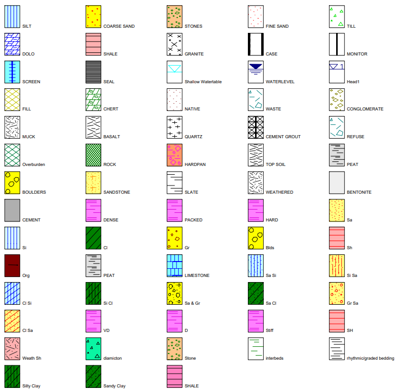*Figure 3* Figure 3: Lithology Legend.

Other perceived biases and patterns were identified during the geological surface refinement process. As most drillers are hired simply to find water, they frequently stop drilling as soon as they encounter a significant aquifer zone. Since tapping into the top few metres of a significant aquifer is all that is necessary to meet the needs of most domestic well owners, very little of the permeable aquifer material is sampled and documented within the driller’s logs. As a result, the majority of driller’s logs are typically a record of aquitard materials, with only the bottom-most screened sand or gravel unit representative of aquifer material. Despite these biases, highly significant patterns were identified within the logs, as discussed in the following sections.

Overview of the Interpretation Process

To analyze the geologic data, and geophysical and hydrogeologic indicators, and build the 3D geologic model, different types of data are used. These data are displayed on cross section for visualization as well as interpretation. The data types include: geologic descriptions from all boreholes (also displaying GSC auto-interpreted lithologies), well-screen elevations and water levels. One of the first tasks in the interpretation process is making geologic formation picks on boreholes displayed on cross sections. These picks are stored in the database for later use in the interpolation of geologic surfaces.

In addition to geologic picks, three-dimensional polylines are drawn during the interpretation process. Polylines, which are lines of contact between different geologic units, are used to control and constrain the process of geologic surface generation. Polylines are typically added in a direction perpendicular or parallel to the axis of interpreted channels or valley features. Each polyline is assigned to a geologic unit, and the individual vertex points in each polyline are then included (along with the geologic picks at boreholes) in the interpretation process (largely kriging) for that particular unit. For example, the drainage pattern in bedrock valley systems is created by adding polylines down the inferred thalweg cross section. The truncation and pinch out of layers at the edges of tunnel channels was defined using polylines perpendicular to the axis of the channel feature. Plan view manual contouring was also integrated as necessary. Surficial geophysics data (seismic lines) are also used.

Figure 4 presents a sample cross section and shows how three-dimensional polylines were used to constrain tunnel channel geometry between borehole locations. The thin black lines in the figure that generally follow the unit boundaries are the constraint polylines. These constraint lines, together with the borehole picks, produce the unit boundaries (final interpolated units are show as solid color filled zones).

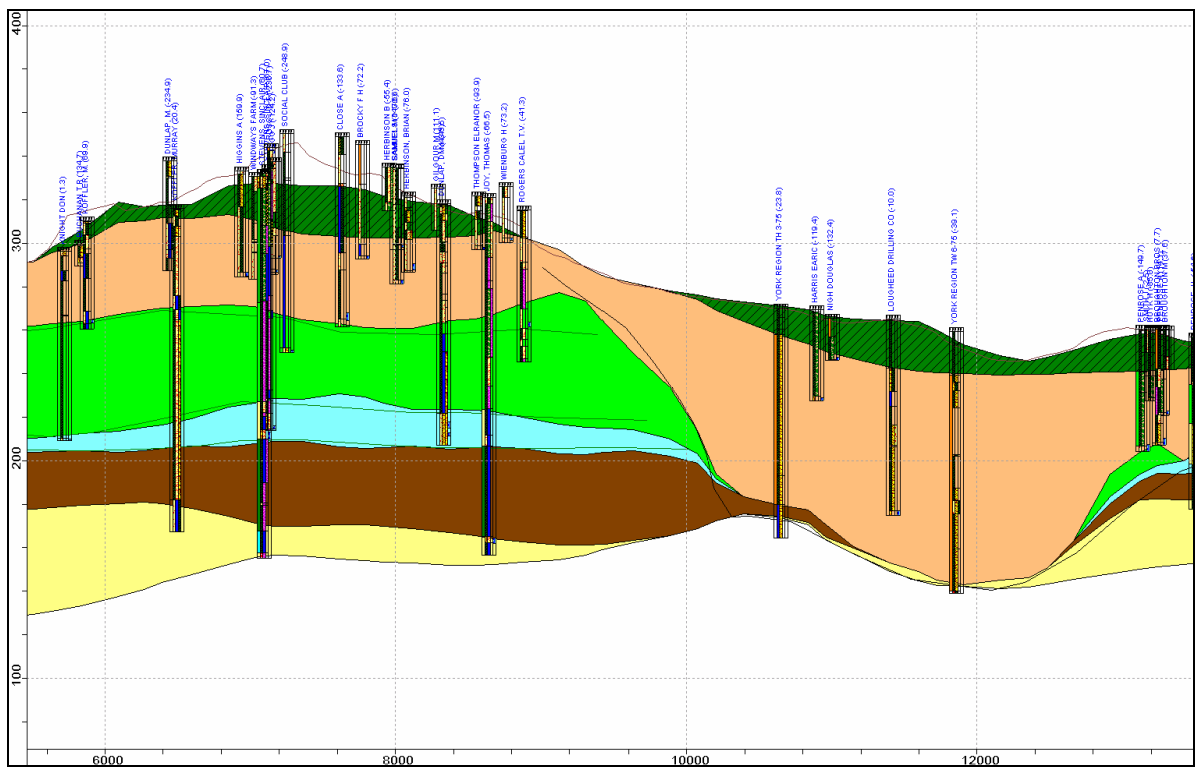*Figure 4* Figure 4: Polylines on cross section used to constrain the geologic unit interpretation between borehole locations.

Interpretation Methodology

Development of the hydrostratigraphic surfaces involves an iterative process of interpretation, gridding and refinement. Layer elevations need to be evaluated when new data becomes available. Elements of the GSC’s rules-based approach to the generation of the stratigraphic surfaces (Logan et al., 2001) are incorporated into the hydrostratigraphic interpretation methodology. The main interpretive methodologies used were:

Geologic picking at boreholes and outcrops;
Three-dimensional constraint polylines;
Push-down locations;
Interpolation of geologic surfaces and variogram analyses; and
Post-processing constraints.

Each of these tasks is described in more detail below.

Step 1: Geologic Picking

Hydrostratigraphic units were picked on thousands of cross sections through the ORM area. These cross sections were viewed, at minimum, along every concession road, which are spaced approximately every 2 km. In more complex areas, cross sections were spaced at 100 to 500 m. Over 800,000 geologic layer picks have been made in boreholes and outcrops (e.g., Scarborough Bluffs, river sections) along these cross sections. Key patterns in the drillers logs emerged during this process and were highlighted using characteristic lithology symbols and colors. An important part of the display was the optimization of certain colours with specific MECP geological descriptors, thereby allowing specific patterns in the material codes to be identified. Some of the important patterns include:

Hardness: the terms “dense”, “hard”, and “packed” is used interchangeably by different drillers. Intervals with these terms are colour coded pink on section. These descriptors appear to be commonly applied to the Newmarket Till. The bright pink colour is therefore used as a guide to identify this unit;
Clay+ stones or Clay+ gravel: The combination of clay and stones (or clay and gravel) has also emerged as a reliable till indicator. In this case clay is the primary material and stones/gravel is the secondary material;
Coarse material + Well Screen: Coarse-grained material alone (i.e., sand) cannot always be assumed to be representative of a good aquifer. In many cases the sand might be quite silty. Sand, combined with a well screen, however, is considered more likely to be representative of a good aquifer;
Well-screen position: In many cases well screens are clustered at a particular depth position, suggesting a good aquifer zone;
Well material similarity and detail patterns: The visual comparison of materials from a group of wells could, in many cases, lead to a better and more reliable interpretation. The noise and variability in the individual well descriptions could be visually filtered to identify a formation contact. A related issue was the level of descriptive detail in an individual well. For example, wells with too few material codes or long sections of very simple descriptions were, in some cases, considered “suspect” (suggesting that the driller was not attentive to the geological changes that were present); and
Silt + a lack of ‘hard’ material code: The GSC suggested (Russell et al., 1998) that in many cases clay materials identified by drillers were actually silt. However, where silt was described in the MECP logs, it was observed that there was a link between the location of these wells and the location of potential tunnel channels. This correlation, especially where the term “hard” as a material modifier was absent, led to a general interpretation that “silt“ was a potential indicator of tunnel channel sediments.

Step 2: Addition of 3D Polyline Constraints

During the cross section interpretation process, 3D polylines were added manually. Each node (or vertex point) along a polyline essentially represents a geologic pick in an area where no wells exist (in total, over 80,000 polyline nodes have been added). These polylines ensured the continuity of geologic structures, particularly in areas where there is a lack of borehole data. Polylines were also used to help constrain push-down conditions (described below).

Polylines were used to define both the base and the width of bedrock valley systems. A combination of deep bedrock wells and deep push-down wells were used to initially define the position of the bedrock valley systems. The shape of the valley was then defined with additional 3D polylines. With limited data in the deep valley systems, particularly the main branch of the Laurentian trough, some assumptions had to be made about the channel width and the slope of the valley walls. Modern analogs were reviewed, including the Niagara River (the Laurentian was suspected to be of a similar size and flow rate). Bronte Creek and 16 Mile Creek, which are relatively deeply incised into the Queenston Shale, and the Credit River were also considered.

The primary question was whether the river would incise deeply into the soft shale, or would the river meander and undermine the valley walls, resulting in a shallow, broad valley. Evidence for both conditions was found, and a basic valley width for the main channel was assumed to be approximately 4 km. Initially polylines were drawn along the thalweg of the valley. Several sets of parallel polylines were then drawn on both sides of the thalweg line and positioned at successively higher elevations to shape the valley to this valley feature. The resulting bedrock surface was checked and modified based on the well data. A seismic survey across the main channel near Schomberg suggests that the channel is at least 4-km wide (Davies et al., 2008). The width of tributaries was evaluated on a case-by-case basis and conformed to local well data. Care was also taken to ensure that the tributaries also correctly hydrologically connected into the main Laurentian channel.

North of the Oak Ridges Moraine, the high-resolution DEM was used as an additional source of information when interpreting the tunnel channels. Constraint polylines were used to extend the surficial expression of the tunnel channels down into the subsurface. However, depth control in this area was limited due to the paucity of data. In the case of the tunnel channels, interpretation lines perpendicular to the channel were drawn that truncated units (e.g., Newmarket Till, Thorncliffe Formation, etc.) at the edges of the inferred channel. The depth of the channels (and the polylines that shape the valleys) was determined by looking for wells with geological intervals that were discontinuous with wells outside of channel areas. In addition, a coarse-grained aquifer within the valley was also sought as a marker that might indicate the coarse depositional phase that is typical at the base of the channel sediment infill which are characterized as fining-upward sequences.

In summary, polylines provide an important control over the interpolation process, however, they need to be used carefully and only where necessary. Verification of the layer geometry is ongoing through both drilling and seismic surveys across the study area. With time, polyline constraints can be removed as data is collected and substituted.

Step 3: Push-Down Check

A push-down condition exists when a borehole partially penetrates a geologic unit: the next lower unit must exist below the bottom of the partially penetrating well, but how far below is unknown. Handling of push-down conditions is particularly important to the interpretation of the bedrock surface because of the sparseness of the data and the potentially strong influence of the Laurentian River valley system. For the bedrock surface, a push-down condition occurs where a deep well does not encounter bedrock. At this location, the bedrock surface must be lower than the bottom of this non-bedrock borehole and therefore, the bedrock surface must be pushed down below the base of that well at this location, even though the bedrock was not encountered at this location.

Deep push-down wells are used both before and after polyline drawing. Bedrock wells and deep push-down wells aree reviewed to initially identify the bedrock valley thalweg locations. Once the thalwegs are defined (as outlined above), additional push-down checks are performed to ensure that these deep, non-bedrock wells were fully integrated into the surface generation process.

Specific display techniques were used to help visualize the push-down conditions. Sediment boreholes (e.g., those that do not encounter bedrock) are plotted on a plan-view map with the elevation of the bottom depth represented by scaled and color-coded symbols. This allows deep push-down wells to appear on the map as large, bright symbols. Bedrock valley thalwegs are then interpreted on plan view, and cross sections are generated along those thalwegs. Polylines are added to the thalweg cross sections to ensure that the bedrock surface correctly represented the decreasing elevation along each valley.

Other push-down surface checks are performed in a manner similar to the GSC methodology (Logan et al., 2001). The following steps are used:

Bedrock picks are made at all wells that intercept bedrock;
The initial bedrock surface was interpolated using all bedrock picks;
The non-bedrock (sediment) wells were evaluated by plotting them on plan view with a bottom-hole elevation represented by scaled and color coded symbols;
Using the initially interpolated bedrock surface and the non-bedrock wells, bedrock valleys are identified and bedrock valley thalwegs are drawn on plan view;
Cross-sections are generated along the bedrock valley thalwegs and bedrock polylines are drawn on-section to represent the bedrock surface. The polylines are drawn to connect the bedrock picks and to ensure that the bedrock surface was beneath the deep non-bedrock wells. The lines are also drawn to ensure that the bedrock surface correctly represents the decreasing elevation of a fluvially eroded valley system;
The secondary bedrock surface was then interpolated using the bedrock picks at the bedrock wells and the vertex points of the bedrock surface polylines that were created along the bedrock valley thalwegs;
This surface is then checked against the non-bedrock wells to see whether any of the non-bedrock wells intersected the secondary bedrock surface;
Where non-bedrock wells are deeper than the secondary bedrock surface the elevation of the well bottom is added as an additional bedrock point to push down the final bedrock surface;
Additional polylines are added on cross-sections parallel to the bedrock valley thalwegs to better shape the bedrock valleys; and
The final bedrock surface is interpolated using all of the above: bedrock picks; polyline vertex points; and the elevation of the bottom of deep non-bedrock wells that pushed down the bedrock surface.

Step 4: Variogram Analyses and Interpolation

Once the picking, polylines and push-down analyses are complete, the geologic surfaces are generated by interpolating the point data to a regular grid. This project makes use of an interpolation method called kriging, which is a distance-weighted averaging technique whereby a system of linear equations is solved using coefficients that are obtained from a variogram analysis. At each cell in the regular grid, a search is conducted for the nearest data points to the centre of that cell. Typically, the nearest 32 points are used to interpolate a value for that grid cell. The interpolated value at each cell centre is based on a theoretical variogram that is used to estimate the relative importance of nearby data points versus those that are further away. In other words, data points that are closer to a grid cell will be weighted higher than data points that are farther from that grid cell during the interpolation process. The result is a gridded geologic surface where every grid cell has an interpolated value for elevation. This process is repeated for each geologic surface.

Step 5: Rules-Based Post Processing

Finally, the surfaces are crosschecked using a series of rules. The rules ensured, for example, that the interpolated layers did not cross one another. The rules were developed and applied in an order that reflected the distinctive characteristics of each hydrostratigraphic interface (i.e., unconformity, etc.) and the confidence and distinctiveness of the lithologic signature. For example, the ground surface was assigned the highest level of confidence, followed by the bedrock surface, top of the Newmarket Till, and then the remaining units. The following were some of the geologic surface post-processing rules:

If bedrock elevation lies above ground surface, then set bedrock elevation to ground surface;
If the top of Newmarket Till elevation is above ground surface, then set top of Newmarket Till elevation to ground surface;
If the top of Newmarket Till elevation is below bedrock elevation, then set top of Newmarket Till elevation to bedrock elevation;
If top of Thorncliffe Formation elevation is above the top of Newmarket Till , then set top of Thorncliffe Formation elevation to top of Newmarket Till elevation;
If top of Thorncliffe Formation elevation is below bedrock, then set top of Thorncliffe Formation elevation to bedrock elevation;
If top of Sunnybrook Drift elevation is above Top of Thorncliffe Formation elevation, then set top of Sunnybrook Drift elevation to top of Thorncliffe Formation elevation; and
etc.

The order in which these rules are processed is important, as each surface check relied on the preceeding checks and constrants. The approach is not a top-down correction. For example, constraining the Halton Till is one of the last checks performed.

Other geologic surface cross checks are included, including reconciliation with the surficial geology units. Hydrogeologic indicators can provide important information regarding geologic layer extent and integrity. For example vertical hydraulic gradient changes can indicate thinning or absence of geologic layers that function as aquitards (till, silt, clay). Mapping of cold water fishery locations may indicate the presence of aquifer outcrops along a stream reach.

Conclusions

The ongoing development of a three-dimensional geologic model at the scale of the Oak Ridges Moraine is a complex, time-consuming task. A key component of this task is layer picking, which requires a concerted effort to understand existing conceptual geologic models and adapt and refine them as necessary. The construction process is complicated by the low-quality and conflicting information contained in the MECP well database.

The geologic surfaces produced through this study and provided by the ORMGP are continually upgraded as new data, knowledge and understanding are acquired. As such, these surfaces will be in need of continual testing and improvement into the future. Although every effort was made to ensure that the geologic layers, and by extension hydrostratigraphic layers, developed are consistent with the data and current conceptual knowledge, the area covered is too large to be able to go into detail everywhere. This testing can only be conducted over time by various practitioners. The concept of continual improvement, particularly in regards to the conceptual model of flow system understanding, is the philosophy of the Oak Ridges Moraine Groundwater Program.

References

Beatty and Associates. 2003. Updating of the MOE Water Well Record Database for the Regions of York, Peel and Durham. Prepared for York Peel Durham Groundwater Strategy STudy Management Team. 300 p.

Davies, S., Holysh, S., and Sharpe, D.R. 2008. An investigation of the buried bedrock valley aquifer system in the Schomberg area of southern Ontario. Ontario Geological Survey, Groundwater Resources Study 8, 30p.

Earthfx Inc. 2006. Groundwater Modelling of the Oak Ridges Moraine Area. Prepared for the York Peel Durham Toronto (YPDT) Conservation Authorities Moraine Coalition (CAMC) Groundwater Management Study. CAMC/YPDT Technical Report Number 01-06.

Gerber, R.E., Sharpe, D.R., Russell, H.A.J., Holysh, S., and Khazaei, Esmaeil. Conceptual hydrogeological model of the Yonge Street Aquifer, south-central Ontario: a glaciofluvial channel-fan setting. Canadian Journal of Earth Sciences, 55, 730-767.

Karrow, P.F. 1967. Pleistocene Geology of the Scarborough Area. Ontario Geological Survey Report 46, 108p.

Logan, C., Russell, H.A.J., and Sharpe, D.R. 2001. Regional three-dimensional stratigraphic modellingof the Oak Ridges Moraine area, southern Ontario. Geological Survey of Canada Current Research 2001-D1.

Russell, H.A.J., Brennand, T.A., Logan, C., and Sharpe, D.R. 1998. Standardization and assessment of geological descriptions from water well records, Greater Toronto and Oak Ridges Moraine areas, southern Ontario. In Current Research 1998-E, Geological Survey of Canada, p. 89-102.

Sharpe, D.R., Dyke, L.D., Good, R.L., Gorrell, G., Hinton, M.J., Hunter, J.A., and Russell, H.A.J. 2003. GSC High-quality borehole, “Golden Spike”, data Oak Ridges Moraine, southern Ontario. Geological Survey of Canada, Open File 1670, 21 p.

Sharpe, D.R., Pullan, S.E., and Gorrell, G. 2011. Geology of the Aurora high-quality stratigraphic reference site and significance to the Yonge Street buried valley aquifer, Ontario. Geological Survey of Canada, Current Research 2011-1, 20p. doi:10.4095/286269.

Sharpe, D.R., Pugin, A.J.M., and Russell, H.A.J. 2018. Geological framework of the Laurentian trough aquifer system, southern Ontario. Canadian Journal of Earth Sciences, 55, 677-708.