Automated Recession Coefficient

Recession Coefficient

Automated stream flow (linear decay) recession coefficient computation:

The stream flow recession coefficient (k), describes the withdrawal of water from storage within the watershed (Linsley et.al., 1975). The recession coefficient is a means of determining the amount baseflow recedes after a given period of time:

\[b_t=kb_{t-1}\]

where $b_{t-1}$ represents the stream flow calculated at one time step prior to $b_t$. (Note, this assumes that total flow measurements are reported at equal time intervals, when unequal intervals are used, k∆t must be used, where ∆t is the time interval between successive b calculations relative to the time step k was calculated at.)

By plotting $b_{t-1}$ vs. $b_t$, the recession coefficient can be determined by finding a linear function (that crosses the origin) such that k is equivalent to the function’s slope. The linear function must envelope the scatter where $b_{t-1}/b_t \to 1.0$. The reasoning here is that where the difference between $b_{t-1}$ and $b_t$ is minimized, then those stream flow values are most-likely solely composed of baseflow, i.e., “the withdrawal of water from storage within the watershed” (Linsley et.al., 1975). Where $b_{t-1}/b_t < 1.0$, it is assumed that stream flow has a larger runoff component, and thus cannot be considered entirely as “baseflow”.

The recession coefficient is computed automatically using an iterative procedure whereby the recession curve is positioned to envelope the log-transformed discharge data versus subsequent discharge, on the condition that the former exceeds the latter.

Note:

By updating the plot to a user-defined stream flow recession coefficient, all $k$-dependent calculations used on the sHydrology web app will be affected; otherwise the automated recession coefficient is used by default.

Automated first-order (inverse) hyperbolic stream flow recession coefficient computation:

An alternative variant to the recession coefficient that assumes that stream flow follows an inverse hyperbolic function of the form:

\[\frac{1}{Q}-\frac{1}{Q_0}=\frac{t}{m}\]

where $1/Q$ is the inverse discharge and $1/Q_0$ is the inverse of discharge at the beginning of a period of stream flow recession. The inverse of the slope of this function yields a first-cut estimate of the $m$ parameter used in TOPMODEL (Beven and Kirkby, 1979).

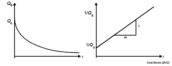
This equation is solved by isolating a number of recession events that appear to fit a similar trend. These inverted stream flow recession events are then plotted against the duration of the event and a final linear regression model is determined. The regression model should only be used when it appears that the underlying recession curves are roughly parallel to the final regression line.

References

Beven, K.J., M.J. Kirkby, 1979. A physically based, variable contributing area model of basin hydrology. Hydrological Sciences Bulletin 24(1): 43-69.

Beven, K.J., 2012. Rainfall-Runoff modelling: the primer, 2\textsuperscript{nd} ed. John Wiley & Sons, Ltd. 457pp.

Linsley, R.K., M.A. Kohler, J.L.H. Paulhus, 1975. Hydrology for Engineers 2^nd ed. McGraw-Hill. 482pp.