Water Budget Model

Soil moisture accounting

The so-called explicit soil moisture accounting (SMA—Todini and Wallis, 1977; O’Connell, 1991) algorithm is used to compute the water balance, and here it is intentionally simplified.

Vertical integration

Where this conceptualization differs from typical SMA schemes is that here there is no distinction made among a variety of storage reservoirs commonly conceptualized in established models. For example, all of interception storage, depression storage and soil storage (i.e., soil moisture below field capacity) is assumed representative by a single aggregate store, thus reducing model parameterization. This conceptualization is allowed by the fact that this model is intended for regional-scale application $(\gg1000\text{ km²})$ at a high spatial resolution $(\text{i.e., }50\times 50\text{ m² cells})$. Users must consider the results of the model from a “bird’s-eye view,” where water retained at surface is indistinguishable from the many stores typically conceptualized in hydrological models.

The SMA’s overall water balance is simply:

\[\Delta S = P-E-R-G,\]

where $\Delta S$ is the change in (moisture) storage, $P$ is “active” precipitation (which includes direct inputs rainfall $+$ snowmelt and indirect inputs such as runoff originating from upslope areas), which is the source of water to the grid cell. $E$ is total evaporation (transpiration $+$ evaporation from soil and interception stores), $G$ is net groundwater recharge (meaning $G<0$ accounts for groundwater discharge), $R$ is excess water that is allowed to translate laterally (runoff). All of $E$, $R$, and $G$ are dependent on moisture storage $(S)$ and $S_\text{max}$: the water storage capacity of the grid cell. Both $E$ and $G$ have functional relationships to $S$ and $S_\text{max}$, and are dependent on other variables, whereas $R$ only occurs when there is excess water remaining $(\text{i.e., }S>S_\text{max})$, strictly speaking:

\[\Delta S = \underbrace{Y_a+B}_{\substack{\text{sources}}} - \underbrace{f\left(E_a,K_\text{sat},S,S_\text{max}\right)}_{\text{sinks}} - \underbrace{R|_{S>S_\text{max}}}_{\text{excess}}\]

see glossary

SMA Reservoirs

Every model cell consists of a retention reservoir $S$ (where water is held locally that has the potential to drain but is still considered “mobile” in that if conditions are met, lateral movement would occur). The reservoir has a predefined capacity and susceptible to evaporation loss. In addition, any number of cells can be grouped which share a semi-infinite conceptual groundwater store $(S_g)$.

Although conceptual, storage capacities are related to common hydrological concepts, for instance:

\[S_\text{max}=\theta_\text{fc} z_\text{ext}+F_\text{imp} h_\text{dep}+F_\text{can} h_\text{can}\cdot\text{LAI}\]

where $\phi$ and $\theta_\text{fc}$ are the water contents at saturation (porosity) and field capacity, respectively; $F_\text{imp}$ and $F_\text{can}$ are the fractional cell coverage of impervious area and tree canopy, respectively; $h_\text{dep}$ and $h_\text{can}$ are the capacities of impervious depression and interception stores, respectively; $\text{LAI}$ is the leaf area index and $z_\text{ext}$ is the extinction depth (i.e., the depth of which evaporative loss becomes negligible). Change in storage at any cell at any time is defined by:

\[\Delta S=y_a+k_\text{in}+b-\left(a+g+k_\text{out}\right),\]

where $y_a$ is atmospheric yield (rainfall + snowmelt), $k = q\frac{\Delta t}{w}$ is the volumetric discharge in $(_\text{in})$ and out $(_\text{out})$ of the grid cell and $f_k$ is the volume of mobile storage infiltrating the soil zone; all units are [m]. (Note that groundwater discharge to streams—$b$—only occurs at stream cells and is only a gaining term.) Also note that $k_\text{out}$ only occurs when water stored in $S_k$ exceeds its capacity.

Groundwater recharge

Groundwater recharge at any given cell is computed when there is surface water in excess $(S^+=S-S_\text{max}>0)$:

\[g=S^+\left[1-\exp\left(\frac{-K_\text{sat}}{L}\Delta t\right)\right].\]

It is important that the second term of the groundwater recharge equation remain to control so-called “cascade towers” which occur when confluences in the cascade network create unrealistically high stages. (This is mainly a consequence of the simplicity of the overland flow scheme applied here—normally, the pressure term in the shallow water equations provides this control physically.) Here the interface length $L=1\text{ mm}$ globally an gives the function form (at $\Delta t=21600 \text{ sec}$).

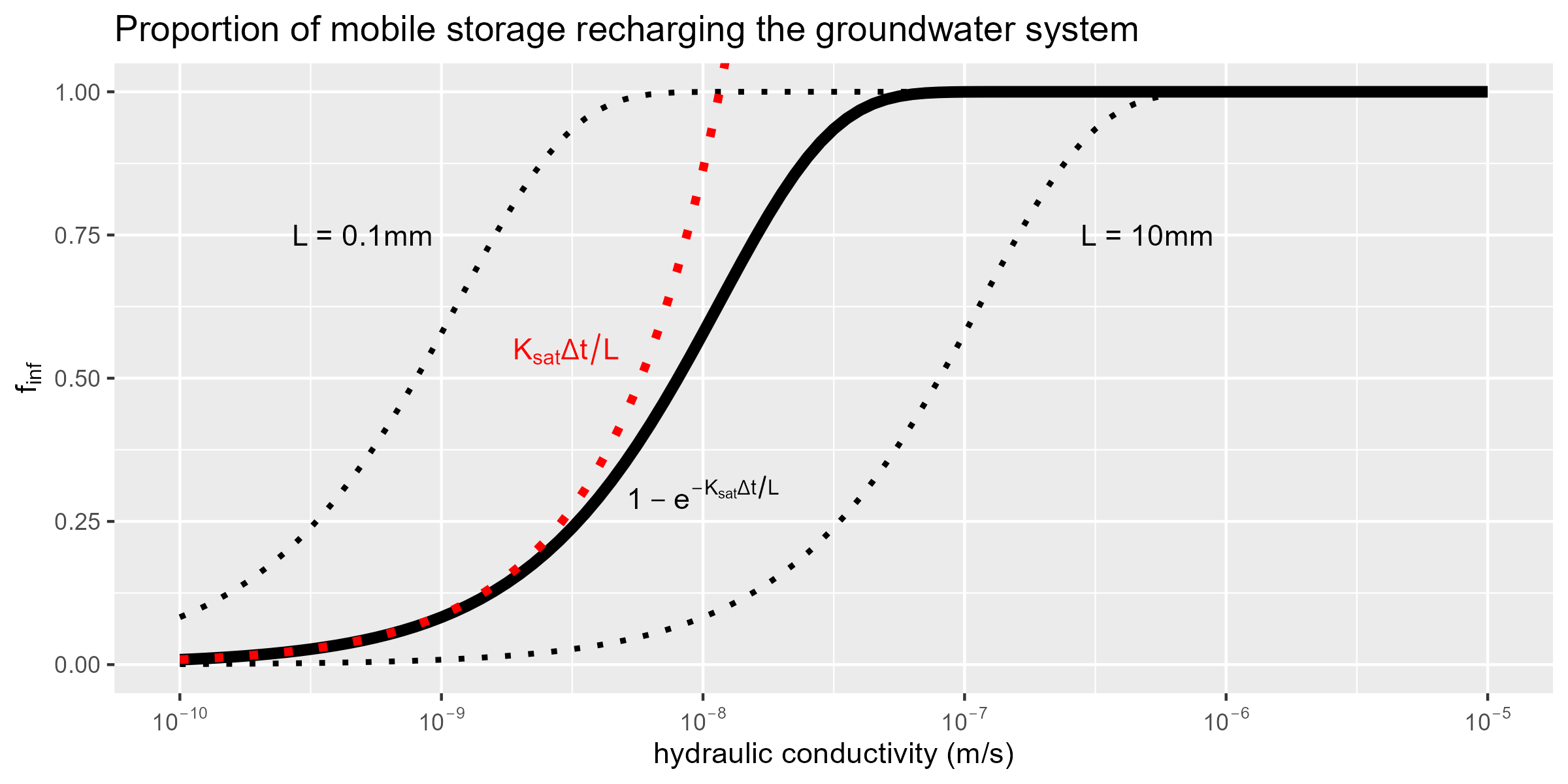
Visual interpretation of the above function. Characteristic length $L$ can clearly be used as a scaling factor, showing here how it varies from $L=1\text{ mm}$. $(\Delta t=86400 \text{ sec}.)$