Water Budget Model

Shallow groundwater model

Typically, the handling of groundwater in rainfall-runoff models involves the use of a groundwater storage reservoir with a linear/exponential decay function. When calibrating these models to long-term stream flow records, this model structure can be quite successful at matching baseflow recession. Given its success and it obvious simplicity, the linear decay groundwater storage model is widely used when the modelling objective is to calibrate to stream flow gauging stations. However, implied in the linear decay groundwater storage model is that the model is “lumped”, meaning that groundwater recharge is assumed uniformly distributed basin-wide, or among common hydrologic response units (HRUs). It also implies that water movement across the surface-subsurface interface is unidirectionally down, meaning there no possibility of groundwater feedback from shallow water tables reducing land surface storage capacity.

Consequently, lumped modelling means that catchment topography is neglected, which has a large role in distributing recharge, both in terms of focused recharge at overland flow convergence points and rejected recharge where the groundwater table is at or above ground surface. For the purpose of this model, which is primarily intended for distributed recharge estimation, the linear decay groundwater storage model on its own will not suffice.

Integrated groundwater-surface water flow models do allow for groundwater feedback as flow across the ground surface interface depend on head gradients that vary spatially. Arguably this is the most “realistic” approach but it comes a grave computational expense (read: long model run times).

TOPMODEL

The groundwater model structure employed here follows the TOPMODEL structure of Beven and Kirkby (1979).

TOPMODEL employs a distribution function that projects predicted groundwater discharge at surface from a simple groundwater storage reservoir. The distribution function is referred to as the “soil-topologic index” (Beven, 1986) that considers distributed surficial material properties, land surface gradients and upslope contributing areas. TOPMODEL does not explicitly model integrated groundwater/surface water processes, however it does provide the ability, albeit an indirect one, to include the influence of near-surface watertables distributed in space. Most importantly, low-lying areas close to drainage features will be prevented from accepting recharge resulting in saturated overland flow conditions.

Assumptions to TOPMODEL are that the groundwater reservoir is lumped meaning it is equivalently and instantaneously connected over its entire spatial extent. This assumption implies that recharge computed to a groundwater reservoir is uniformly applied to its water table. The groundwater reservoir is thought to be a shallow, single-layered, semi-infinite unconfined aquifer whose hydraulic gradient can be approximated by local surface slope.

Lateral (downslope) transmissivity $(T)$ is then assumed to scale exponentially with soil moisture deficit $(D)$ by:

\[T = T_o\exp{\left(\frac{-D}{m}\right)}, % T = T_o\exp{\left(\frac{-D}{m}\right)} = T_o\exp{\left(\frac{-\phi z_\text{wt}}{m}\right)},\]

where $T_o=wK_\text{sat}$ is the saturated lateral transmissivity perpendicular to an iso-potential contour of unit length $(w)$ [m²/s] that occurs when no soil moisture deficit exists (i.e., $D=0$–meaning the water table is at ground surface) and $m$ is a scaling factor with the dimension of length [m]. Consequently, recharge computed in the distributed sense is aggregated when added to the lumped reservoir. Discharge to surface is spatially distributed according to the soil-topographic index. For additional discussion on theory and assumptions, please refer to Beven et.al., (1995), Ambroise et.al., (1996) and Beven (2012).

Under the assumption that the groundwater reservoir is unconfined lends the model the ability to predict the depth to the water table $(z_{wt})$ when porosity $(\phi)$ is known:

\[D=\phi z_{wt} \qquad\text{when}\quad D>0.\]

At the ORMGP regional scale, multiple TOPMODEL reservoirs have been established to represent groundwater dynamics in greater physiographic regions, where it is assumed that material properties are functionally similar and groundwater dynamics are locally in sync.

Distributed across $n$ cells

Groundwater discharge estimates from each TOPMODEL reservoir instantaneously contributes lateral discharge to model grid cell $i$ according to Darcy’s law:

\[q_i = T_o S_0\exp(-D_i/m),\]

where $q_i$ is interpreted here as groundwater discharge per unit length of stream/iso-potential contour [m²/s] at grid cell $i$, and $S_0$ is the local surface slope [L/L] in the downslope direction, assumed representative of the saturated zone’s hydraulic gradient.

Note that in Beven and Kirkby’s (1979), and many subsequent papers referring to TOPMODEL, the term $\tan\beta$ is often used, where $\beta$ is the local surface slope angle in the downslope direction. Here, we are replacing this term with the term $S_0$, to avoid confusion.

The sub-surface storage deficit $(D_i)$ at grid cell $i$ is determined using the distribution function:

\[D_i = \overline{D} + m \left(\gamma - \zeta_i\right),\]

where $\overline{D}$ is the mean deficit of all cells. $\zeta_i$ is the soil-topographic index at cell $i$ defined by:

\[\zeta=\ln\left(\frac{a}{T_o S_0}\right)\]

and $a_i$ is the unit contributing area defined here as the total contributing area to cell $i$ divided by the cell’s width $w$. The catchment average soil-topographic index:

\[\gamma = \frac{1}{A}\sum_i A_i\zeta_i,\]

where $A$ and $A_i$ is the sub-watershed and grid cell areas, respectively.

Groundwater exchange

Ponded conditions

Although plausible, TOPMODEL can be allowed to have negative local soil moisture deficits $(\text{i.e., } D_i<0)$, meaning that water has ponded and overland flow is being considered. For the current model however, ponded water and overland flow are being handled by an explicit soil moisture accounting (SMA) scheme and a lateral shallow water movement module, respectively.

Conditions where $D_i<0$ for any grid cell will have its excess water $(x_i=-D_i)$ added to the SMA system and $D_i$ will be reset to zero. Under these conditions, no recharge will occur at this cell as upward gradients are being simulated.

This exchange, in addition to groundwater discharge to streams, represents the interaction the groundwater system has on the surface, distributed in space. With recharge $(g)$ at the model grid cell computed by the SMA when deficits are present $(D_i<0)$, net basin groundwater exchange $(G)$ is determined by:

\[G = \sum_i(g-x)_i.\]

Therefore, when $G>0$, the lumped groundwater reservoir is being recharged.

Groundwater discharge to streams

Baseflow

The volumetric flow rate of groundwater discharge to streams $Q_b$ [m³/s] for the entire model domain is given by:

\[Q_b = \frac{AB}{\Delta t} = \sum_{i=1}^Ml_iq_i,\]

where $B$ is the total groundwater discharge to streams occurring over a time step $\Delta t$ [m/s], $l_i\approx\Omega_i w$ is length of channel in grid cell $i$ [m], here assumed constant and equivalent to the uniform cell width $(w)$ times a sinuosity factor $(\Omega)$, and $M$ is the total number of model cells containing stream channels (termed “stream cells”).

Stream cells were identified as DEM cells having a contributing area greater than a set threshold of 1000 cells $\approx$ 2.5km², rather than being determined from watercourse mapping.

For every stream cell $i$, groundwater flux to the cell $b_i$ [m] over the timestep $\Delta t$ is given by:

\[b_i=\frac{l_iq_i}{A_i}\Delta t=\frac{\Omega_i w q_i}{A_i}\Delta t=b_{0,i}\exp\left(\frac{-D_i}{m}\right) \Delta t, %\qquad i \in \text{streams}\]

where $b_0$ groundwater flux at stream cell $i$ when the watertable is above the channel bed at saturated conditions $(D<0)$ and is defined by:

\[% b_0=\Omega\cdot \frac{T_o\tan\beta}{w}=\Omega\cdot \tan\beta \cdot K_\text{sat} % b_0=\Omega\cdot \tan\beta \cdot K_\text{sat}. b_0=\Omega\cdot S_0 \cdot K_\text{sat}.\]

Finally, groundwater discharge to streams from the groundwater reservoir is computed by:

\[B = \sum_i b_i.\]

Initial conditions

Initial watershed average soil moisture deficit can, in principle, be determined from streamflow records by re-arranging the above equations (Beven, 2012):

\[%\overline{D}_{t=0} = -m \ln\left(\frac{Q_{t=0}}{Q_o}\right), %\overline{D}_{t=0} = -m\left[\gamma +\ln\left(\frac{Q_{t=0}}{\sum_{i=1}^Ml_ia_i}\right)\right], \overline{D}_{t=0} = -m\left[\gamma +\ln\left(\frac{Q_{t=0}}{A}\right)\right],\]

where $Q_{t=0}$ is the measured stream flow known at the beginning of the model run. The parameter $m$ can be pre-determined from baseflow recession analysis (Beven et.al., 1995; Beven, 2012) incorporated into ORMGP R-shiny using:

\[\frac{1}{Q}-\frac{1}{Q_0}=\frac{t}{m}.\]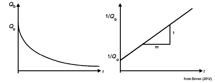

Time stepping

Before every time step, average moisture deficit of every groundwater reservoir is updated at time $t$ by:

\[\overline{D}_t = \frac{1}{A}\sum_i A_i D_i - G_{t-1} + B_{t-1} - Q_{t-1},\]

where $G_{t-1}$ is the total groundwater recharge computed during the previous time step [m], $B_{t-1}$ is the basin-wide (normalized) groundwater discharge to streams, also computed during the previous time step [m], and $Q_{t-1}$ are any additional sources(+)/sinks(-) such as groundwater pumping or exchange between other groundwater reservoirs.

Model-code implementation

It should first be noted that the above formulation is the very similar to the linear decay groundwater storage model. Only here, TOPMODEL allows for an approximation of spatial soil moisture distribution that determines the recharge-runoff distribution, including groundwater feedback–a mechanism instrumental to integrated groundwater surface water modelling.

Rearranging the above terms gives:

\[\delta D_i = \frac{D_i-\overline{D}}{m} = \gamma - \zeta_i,\]

where $\delta D_i$ is the groundwater deficit relative to the regional mean that is independent of time, and therefore can be parameterized. From this, at any time $t$, the local deficit is computed by:

\[D_{i,t} = m\cdot \delta D_i + \overline{D}_t,\]

or with respect to depths to the water table as:

\[z_{wt_{i,t}} = \frac{1}{\phi}\left( m\cdot \delta D_i + \overline{D}_t\right).\]

Groundwater discharge occurs in any saturated areas $(D_i<0)$ and is given by:

\[\begin{align*} b_i = \frac{wq_i}{A_i} = \frac{q_i}{w} &= \frac{T_oS_0\exp(-D_i/m)}{w} \\\\ &= K_\text{sat}S_0\exp(-D_i/m) \end{align*}\]

References

Ambroise, B., K. Beven, J. Freer, 1996. Toward a generalization of the TOPMODEL concepts: Topographic indices of hydrological similarity, Water Resources Research 32(7): pp.2135—2145.

Beven, K.J., 1986. Hillslope runoff processes and flood frequency characteristics. Hillslope Processes, edited by A.D. Abrahams, Allen and Unwin, Winchester, Mass. pp.187—202.

Beven, K.J., R. Lamb, P.F. Quinn, R. Romanowicz, and J. Freer, 1995. TOPMODEL. In Singh V.P. editor, Computer Models of Watershed Hydrology. Water Resources Publications, Highland Ranch, CO: pp. 627—668.

Beven, K.J. and M.J. Kirkby, 1979. A physically based variable contributing area model of basin hydrology. Hydrological Science Bulletin 24(1):43—69.

Beven, K.J., 2012. Rainfall-Runoff modelling: the primer, 2nd ed. John Wiley & Sons, Ltd. 457pp.